
Understanding Cascade Control and Its Applications For HVAC
Miles Ryan, a P.E. at QSEng authored this ASHRAE article published in February 2021.
Most readers familiar with the operation of HVAC systems are aware of the term closed-loop control, oftentimes referred to as just a control loop, closed-loop, or feedback loop. Additionally, many will describe them as PID loops, short for Proportional-Integral-Derivative loops, although this is often not a completely accurate term. Most readers have also probably encountered a variant of closed-loop control called cascade control, although they may not be aware of it.
Cascade control, or cascading control loops1, is a term rarely used in the HVAC industry. In fact, though applications of the concept are discussed, the term itself is not used a single time in ASHRAE Guideline 36 – High-Performance Sequences of Operation for HVAC Systems2. Additionally, there is no universal substitute term for this control approach either. Rather, specifying engineers, temperature controls contractors, commissioning providers, building operators and the like often struggle to explain this concept when implementation of such control logic is encountered. A fundamental understanding of cascade control and the benefits it provides to the operation of HVAC systems is often missing. This results in miscommunication, the leading cause of everything frustrating in the project delivery process. The intent of this article is to explain the theory and common applications of such a control approach in HVAC systems.
Closed-Loop Control Theory
Closed-loop control is a foundational concept in the automation of HVAC systems. The concept is commonly illustrated in diagrams similar to that shown in Figure 1. The goal is to keep the controlled variable at setpoint. Common controlled variables in HVAC applications would be space temperature, return air relative humidity, static pressure in the supply duct, etc. The controlled variable is kept at setpoint by measuring it with a sensing element and relaying that information to the controller. The controller compares that value to setpoint and outputs a control signalto adjust the controlled device accordingly. Adjustments to the controlled device result in changes in the manipulated variable, which have an affect on the process plant. The effect imposed on the process plant needs to be one which brings the controlled variable back toward setpoint. And of course, the controller will know how well it is perfoming since it is constantly getting feedback on how its decisions affect the controlled variable. This continuous feedback loop allows closed-loop control to be effective.
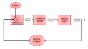
Figure 1: Closed-loop control diagram
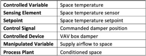
Closed-loop control is utilized all over in HVAC systems. One example would be a pressure-dependent VAV box whose damper position is modulated to maintain space temperature at setpoint. The components of this control loop are identified in Table 1.
Table 1: Closed-loop control: Pressure-dependent VAV box application
This application of closed-loop control quickly points out an inherent issue with this approach. Closed-loop control has tunnel vision, only focusing on the controlled variable and how it can be brought back to setpoint. If the setpoint is thought of as the desired destination, then the value of the manipulated variable is analogous to the speed in which the controlled variable gets there. Speed limits are needed in vehicular applications to ensure safe operation of the vehicle, and they are often needed in HVAC applications as well. Let’s explain.
If the space temperature is above setpoint for an extended period, the damper may go its maximum position. The intent would be for it to provide the maximum design cooling airflow to the space at such instances. However, if the upstream static pressure in the ductwork serving this box is greater than what the system was balanced at, then the space will receive more airflow than intended. This could create drafts, excess noise and may reduce the air system’s ability to provide air to other spaces.
Similarly, if the space is being overcooled, eventually the damper will settle on a minimum position. The intent in these instances would be for the scheduled minimum airflow rate to be provided to the space. If there is higher-than-anticipated upstream static pressure, then more airflow than intended will be provided, further subcooling the space, possibly requiring additional reheat and always wasting energy. If less-than-anticipated upstream static pressure is present, then ventilation requirements may not be met.
Deviations in upstream static pressure reduces the ability of the box to truly operate within its desired range of airflows. The airflow rates these boxes provide are dependent on upstream static pressure. That is why they are referred to as pressure-dependent VAV boxes. Additionally, large fluctuations in the upstream static pressure can reduce the ability of the control loop to hold the controlled variable at setpoint. Deviations in the upstream static pressure would be classified as disturbances to the control loop. There is a more sophisticated variant of closed-loop control which can more quickly identify and adjust for such disturbances. It is called cascade control, and the benefits it provides HVAC systems are often more than what meets the eye.
Cascade Control Theory
Cascade control is often referred to as a “control loop within a control loop.” The end goal is still the same, keep the controlled variable at setpoint. However, now an additional sensing element is placed into the system to measure the manipulated variable, this provides the following benefits:
- Limits can be placed on the values the manipulated variable can operate at.
- Disturbances to the system, which manifest themselves in disruptions to the manipulated variable, are more quickly identified and addressed.
A diagram of the logic is shown in Figure 2.
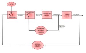
Figure 2: Cascade control diagram*
*The diagram shows two separate controllers; however, each block merely represents a control response to error from set point. Many applications of cascade control have a single physical controller capable of processing both responses.
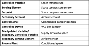
In the pressure-dependent VAV box example above, fluctuations in supply air’s static pressure result in fluctuations in the manipulated variable, the airflow rate. Such a VAV box would be made pressure-independent by adding an airflow sensor. That sensor would measure the manipulated variable (i.e. airflow rate) and prevent it from operating at unacceptable values. This is done by making the manipulated variable a secondary controlled variable within a secondary control loop. The system will measure the manipulated variable (i.e. airflow rate), compare it to an airflow setpoint and adjust the damper position accordingly. However, we will need to adjust that airflow setpoint (the secondary setpoint) when the controlled variable (i.e. space temperature) is not being maintained at its setpoint. Thus, that airflow setpoint will be reset whenever space temperature begins to deviate from its setpoint. The components of the control loop for pressure-independent VAV boxes can be seen in Table 2.
Table 2: Cascade control: Pressure-independent VAV box application
The concept of a pressure-independent VAV box may sound familiar, they are the norm. They ensure the box does not provide more than the maximum design airflow rate. Additionally, such pressure-independent boxes can be used to ensure minimum ventilation requirements are maintained during periods of low or no cooling load on the space. Lastly, large fluctuations in airflow due to variations in upstream static pressure can be identified well before they result in further error from the space temperature setpoint. This further improves the box’s ability to keep the space temperature at setpoint.
Though the theory behind cascade control may seem excessively sophisticated, there are numerous applications of this form of control in conventional HVAC systems today. Several examples are described below with the components of their control loops identified in Table 3.
Conventional Applications
Table 3: Cascade control: Conventional applications**
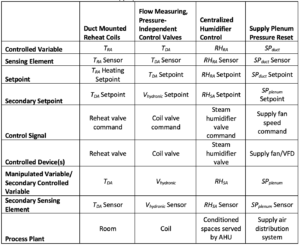
**Definitions in this table: TRA = room air temperature; TDA = discharge air temperature; Vhydronic = hydronic flow rate; RHRA = return air relative humidity; RHSA = supply air relative humidity; SPduct = supply duct static pressure; SPplenum = supply plenum static pressure
Duct Mounted Reheat Coils
Historically, duct mounted reheat coil valves (either located at a VAV box or standalone) were controlled to maintain room temperature directly in closed-loop control. Installing a discharge air temperature sensor downstream of the reheat coil allows for the reheat valve to control to a discharge air temperature setpoint instead. That discharge air temperature setpoint can be reset to maintain the room air temperature at its setpoint.
This approach allows for an upper limit to be placed on the discharge air temperature setpoint. Too warm of discharge air, coupled with a ceiling supply and ceiling return air distribution arrangement, will result in short-circuiting of warm supply air directly into the return grille. This will drive up energy consumption as well as reduce the effectiveness of the HVAC system to heat the space. It is for this reason ASHRAE Standard 90.13 prohibits distribution of supply air more than 20°F (11.1°C) above space temperature setpoint. ASHRAE Standard 62.14 has even tighter requirements to keep the zone air distribution effectiveness value at 1.0. It is for these reasons ASHRAE Guideline 36 dictates controlling the reheat valve to a resetting discharge air temperature setpoint in lieu of controlling directing to the space temperature.2
An additional benefit of this approach would be self-balancing of the hot water system as it helps to prevent more than design hot water flow from passing through the reheat coil.5 Reheat coils are almost always large enough to meet their scheduled discharge air temperature for the scheduled airflow rate. It is when the served space’s heating requirements exceed design values, and the reheat coil is controlling directly to space air temperature, that the reheat valve will fully open and the coil will pull more than its fair share of hot water flow. This is typically seen during morning warmup or at zones that are incapable of meeting their room temperature heating setpoints for any number of reasons.
Flow Measuring Pressure-Independent Control Valves
Installing flow measuring, pressure-independent control valves to serve large AHU coils is becoming more common. Instead of modulating a control valve to track on discharge air temperature directly, an integral flow sensor allows for the valve to instead control to a hydronic flow setpoint. That hydronic flow setpoint will be reset to keep the discharge air temperature at setpoint.
Such an approach allows for the valve to more quickly address fluctuations in hydronic system differential pressure, that is where the term “pressure-independent” comes from. This will allow for tighter control of the discharge air temperature. Additionally, the flow setpoint can be limited to a range, which can be used to prevent the coil from pulling more than its fair share of flow from the system. This allows for self-balancing of the system and can be used to avoid the coil from entering the “saturation region” of its performance curve, a region where large increases in hydronic flow result in a negligible increase in heat transfer at the coil.6 Coils operating in the saturation region are a large contributor to low delta T syndrome.7,8
Centralized Humidifier Control
Direct steam injection humidifiers located at an AHU are often controlled to maintain return air relative humidity at setpoint. It takes time before increases in humidifier output raises the return air relative humidity an appreciable amount. This delay could result in the humidifier output getting too high, saturating the supply air duct which could result in condensate blown out of supply diffusers or a duct mounted high humidity switch disabling the humidifier altogether.
Implementing cascade control where the modulating steam humidifier valve controls to a supply air relative humidity setpoint, which is reset to keep the return air relative humidity at its setpoint, can put limits on the supply air relative humidity to ensure stable operation.
Supply Plenum Pressure Reset
Some air distribution systems have the supply fan control to the static pressure in the supply plenum immediately downstream of the supply fan. This setpoint is reset to keep a supply duct static pressure further down the air distribution system at its setpoint.
The application of cascade control here is primarily for stable control of the supply fan. This places limits on the plenum pressure, which will prevent the fan from ramping up to try and satisfy a duct pressure sensor which may be downstream of a fire damper that has failed shut. Such uncontrolled ramping of the fan speed may take the unit offline due to the tripping of a static pressure safety switch, or possibly blow out a supply duct.
Additionally, the downstream duct’s static pressure sensor is often wired to a separate controller than the AHU controller. If network issues hinder the feedback for that sensor, local control of the supply fan for downstream plenum pressure would result in stable operation until network issues are resolved.
Unconventional Applications – A Case Study
Having a foundational understanding of cascade control will allow one to recognize opportunities for its implementation in unconventional applications as well. Cascade control is appropriate when limits need to be placed on the values the manipulated variable can obtain or when the manipulated variable is subject to disturbances. The previous examples all highlight instances when limits need to be placed on the manipulated variable. The following example details how it can be used to more effectively address system disturbances to improve the controllability of a system.
This author’s firm was asked to investigate inadequate heating at a high-rise condominium complex. Minnesota’s polar vortex of January 2019 resulted in many condos unable to heat above 55°F (12.8°C). The hot water system was of a primary/secondary pumping configuration as shown in Figure 3. The secondary pumps provided heat to downstream finned tube radiation (FTR) and fan coil units (FCU) located in the residences, as well as to a hot water-to-glycol hot water heat exchanger. The glycol hot water solution was then used to heat incoming ventilation air at the makeup air unit (MAU).
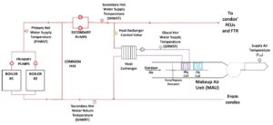
Figure 3: High-rise condominium’s hot water system serving MAU’s heat exchanger and terminal loads
The root causes of insufficient heating were many, but the biggest shortcoming of the system was secondary flow exceeding primary flow. This occurs when secondary flow does not track on load, i.e. the secondary flow remains high even during periods of low heating load. When secondary flow exceeds primary flow, water travels opposite of the intended direction in the common pipe, which results is the secondary hot water supply temperature (SHWST) falling below that of the primary hot water supply temperature (PHWST). Degrading SHWSTs reduces downstream heating mechanisms’ ability to provide heat, which further increases secondary flow, which sends more secondary flow backwards through the common pipe, which in turn further degrades the SHWST. The boilers, which control to PHWST are oblivious to the system’s inability to provide heat to the spaces served. This scenario has been astutely referred to as the “death spiral” in literature discussing low delta T syndrome in chilled water systems.9
The primary reason for excessive secondary flow in the high-rise condominium complex was due to the MAU’s heating sequence of operation. During heating operation, the hot water valve serving the heat exchanger was commanded full open. This resulted in substantially higher glycol hot water supply temperatures (GHWST) than needed. This did not result in overheating of the supply air however, as the MAU’s face and bypass dampers were modulated to effectively maintain the supply air temperature (TSA) at setpoint.
To bring the secondary flow rate below the primary flow rate, the heating sequence for the MAU was adjusted as follows: During heating operation, the face and bypass damper goes full face and the heat exchanger’s control valve modulates to maintain the TSA at setpoint.
This strategy would minimize the amount of hot water flow needed at the heat exchanger to meet the heating requirements of the MAU.
Implementing this strategy immediately resulted in a reduction in secondary flow and the SHWST rose to match that of the PHWST. This improved downstream FTR sections’ ability to heat the condos. It was quickly realized however that this closed-loop control was insufficient for TSA control of the MAU. No amount of tuning could get away from large temperature fluctuations around the TSA setpoint (see Figure 4). These fluctuations in TSA were traced back to fluctuations in the PHWST. The boiler plant consisted of two atmospheric boilers, each with two stages of heat. Bringing on an additional stage of heat at times would raise the PHWST (and SHWST) 30°F (16.7°C) or more in 3 minutes. Disabling a stage of heat would at times drop the supply temperature at about the same rate.
These undesirable fluctuations in SHWST resulted in unintended fluctuations in the GHWST. The fluctuations in GHWST resulted in large deviations in TSA from setpoint. The system needed a way to identify and react to these disturbances before they so drastically affected the TSA. Cascade control was required.
The MAU heating sequence was then adjusted a second time. The hot water valve at the heat exchanger now modulates to keep the GHWST at setpoint, which is reset to keep the TSA at its setpoint. The moment this cascade control logic was implemented can be seen in Figure 4. Oscillations in supply air temperature around its setpoint were immediately reduced to less than 1°F in amplitude. Ongoing monitoring of the system has confirmed this level of performance has been sustained.
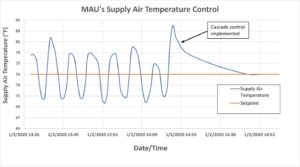
Figure 4: MAU’s supply air temperature control improved by cascade control implementation.
Not only did implementing cascade control improve the ability of the system to maintain TSA at setpoint, it was also determined that this unstable control loop was a trigger which had ripple effects elsewhere in the system. Previous hunting of the valve created periods of low load on the heat exchanger followed by periods of high load. Cascade control allows for a steady load on the heat exchanger. Implementing cascade control resulted in smaller fluctuations in the PHWST. Once observed temperature oscillations in the PHWST of 30°F (16.7°C) have been reduced to never more than 12°F (6.7°). This is prime example of how one unstable control loop can have ripple effects into other control loops in the system, a concept which has been detailed in other HVAC applications.10
Conclusion
Cascade control has numerous applications in both conventional and unconventional HVAC systems. However, it is term rarely used nor is it a concept universally understood. This article intends for folks to spend time to understand the concept. It will allow readers to better articulate these sequences in specifications and submittals, comprehend these sequences quicker as well as realize when its application is appropriate. Foundational understanding of this concept will bring value to the project delivery process and ultimately the performance of HVAC systems.
- Montgomery, R., R. McDowall. 2011. Fundamentals of HVAC Control Systems. ASHRAE
- ASHRAE Guideline 36-2018, High-Performance Sequences of Operation for HVAC Systems.
- ANSI/ASHRAE Standard 90.1-2019, Energy Standard for Buildings Except Low-Rise Residential Buildings.
- ANSI/ASHRAE Standard 62.1-2019, Ventilation for Acceptable Indoor Air Quality.
- Taylor, S. J. Stein, G. Paliaga, H. Cheng. 2012. “Dual maximum VAV box control logic.” ASHRAE Journal (12).
- Ryan, M., G. Henze. 2017. “Airside system-type prediction enabled by intelligent pressure independent control valves.” Journal of Architectural Engineering 23(3).
- Thuillard, M., Reider, F., Henze, G. P. 2014. “Energy efficiency strategies for hydronic systems through intelligent actuators.” ASHRAE Transactions. 120(1).
- Henze, G.P., Henry W., Thuillard, M. (2013) “Improving Campus Chilled Water Systems with Intelligent Control Valves: A Field Study.” Proceedings of the 2013 ASCE Architectural Engineering Conference, April 2-5, 2013, State College, PA.
- Energy Design Resources. 1999. CoolTools™ Chilled Water Plant Design Guide.
- Sellars, D. 2004. “Troubleshooting and tweaking air-handling systems.” HPAC Engineering (12).
Ryan is a commissioning engineer at Questions & Solutions Engineering in Chaska, MN as well as a mechanical systems instructor at the Air Force Institute of Technology at Wright-Patterson AFB, OH.